(setq org-babel-default-header-args:R
      '((:session . "org-R")))
For some reason, BigDFT is just impossible to trace in RL with Tau or Scalasca. Either it segfault or it hangs… Surprisingly, it works like a charm with Paraver. Remember we want to compare a RL trace with an SMPI trace. Unfortunately, we haven't found any converter from Paraver files to Tau or OTF or anything that we could later convert to CSV and analyze with R… So I've quickly written a quick and dirty perl script that converts Paraver files to CSV files similar to the ones we obtain with pjdump.
Paraver Conversion and R visualization
Augustin just sent me a typical paraver trace. Let's convert it:
ls paraver_trace/
| EXTRAEParavertracempich.pcf |
| EXTRAEParavertracempich.prv |
| EXTRAEParavertracempich.row |
The pcf file describes events, the row file defines the
cpu/node/thread mapping and the prv is the trace with all events. The
description of the file format is given here
http://pcsostres.ac.upc.edu/eitm/doku.php/paraver:prv
# use strict;
use Data::Dumper;
my $prv_input=$input.".prv";
my $pcf_input=$input.".pcf";

open(OUTPUT,"> $output");

sub parse_pcf {
  my($pcf) = shift;
  my $line;
  my(%state_name, %event_name) ;
  open(INPUT,$pcf) or die "Cannot open $pcf. $!";
  while(defined($line=<INPUT>)) {
     chomp $line;
     if($line =~ /^STATES$/) {
       while((defined($line=<INPUT>)) &&
             ($line =~ /^(\d+)\s+(.*)/g)) {
          $state_name{$1} = $2;
       }
     }
     if($line =~ /^EVENT_TYPE$/) {
       $line=<INPUT>;
       $line =~ /[6|9]\s+(\d+)\s+(.*)/g or next; #E.g. , EVENT_TYPE\n 1    50100001    Send Size in MPI Global OP
       my($id)=$1;
       $event_name{$id}{type} = $2;
       $line=<INPUT>;
       $line =~ /VALUES/g or die;
       while((defined($line=<INPUT>)) &&
             ($line =~ /^(\d+)\s+(.*)/g)) {
          $event_name{$id}{value}{$1} = $2;
       }
     }
  }
#  print Dumper(\%state_name);
#  print Dumper(\%event_name);
  return (\%state_name,\%event_name);
}

sub parse_prv {
  my($prv,$state_name,$event_name) = @_;
  my $line;
  my (%event);

  open(INPUT,$prv);
  my($pcf) = shift;
  while(defined($line=<INPUT>)) {
    chomp $line;
    # State records 1:cpu:appl:task:thread : begin_time:end_time : state
    if($line =~ /^1/) {
      my($sname);
      my($state,$cpu,$appli,$task,$thread,$begin_time,$end_time,$state) =
         split(/:/,$line);
      if($$state_name{$state} =~ /Group/) {
        $line=<INPUT>;
        chomp $line;
        my($event,$ecpu,$eappli,$etask,$ethread,$etime,%event_list) =
           split(/:/,$line);
        (($ecpu eq $cpu) && ($eappli eq $appli) &&
         ($etask eq $task) && ($ethread eq $thread) &&
         ($etime >= $begin_time) && ($etime <= $end_time)) or
        die "Invalid event!";
        $sname = $$event_name{50000002}{value}{$event_list{50000002}};
      } else {
        $sname = $$state_name{$state};
      }
      print OUTPUT "State, $task, MPI_STATE, $begin_time, $end_time, ".
                   ($end_time-$begin_time).", 0, ".
                   $sname."\n";
    }
    # Event records 2:cpu:appl:task:thread : time : event_type:event_value
    if($line =~ /^2/) {
      my($event,$cpu,$appli,$task,$thread,$time,@event_list) =
         split(/:/,$line);
#      print OUTPUT "$time @event_list\n";
    }
  }
}

my($state_name,$event_name) = parse_pcf($pcf_input);
parse_prv($prv_input,$state_name,$event_name);
print "$output";
/tmp/bigdft_8_rl.csv
head /tmp/bigdft_8_rl.csv
| State | 1 | MPISTATE | 0 | 10668 | 10668 | 0 | Not created |
| State | 2 | MPISTATE | 0 | 5118733 | 5118733 | 0 | Not created |
| State | 3 | MPISTATE | 0 | 9374527 | 9374527 | 0 | Not created |
| State | 4 | MPISTATE | 0 | 17510142 | 17510142 | 0 | Not created |
| State | 5 | MPISTATE | 0 | 5989994 | 5989994 | 0 | Not created |
| State | 6 | MPISTATE | 0 | 5737601 | 5737601 | 0 | Not created |
| State | 7 | MPISTATE | 0 | 5866978 | 5866978 | 0 | Not created |
| State | 8 | MPISTATE | 0 | 5891099 | 5891099 | 0 | Not created |
| State | 1 | MPISTATE | 10668 | 25576057 | 25565389 | 0 | Running |
| State | 2 | MPISTATE | 5118733 | 18655258 | 13536525 | 0 | Running |
OK. Conversion seems fine. It's a little messy and some stuff is hardcoded but it does the job. Let's load it in R.
1 2 3 4 5 6 7 8 9 10 11 12 13 14 15 16 17 18 | |
Use suppressPackageStartupMessages to eliminate package startup messages.
  ResourceId Start         End    Duration       Value               Origin
1          1     0 0.000010668 0.000010668 Not created /tmp/bigdft_8_rl.csv
2          2     0 0.005118733 0.005118733 Not created /tmp/bigdft_8_rl.csv
3          3     0 0.009374527 0.009374527 Not created /tmp/bigdft_8_rl.csv
4          4     0 0.017510142 0.017510142 Not created /tmp/bigdft_8_rl.csv
5          5     0 0.005989994 0.005989994 Not created /tmp/bigdft_8_rl.csv
6          6     0 0.005737601 0.005737601 Not created /tmp/bigdft_8_rl.csv
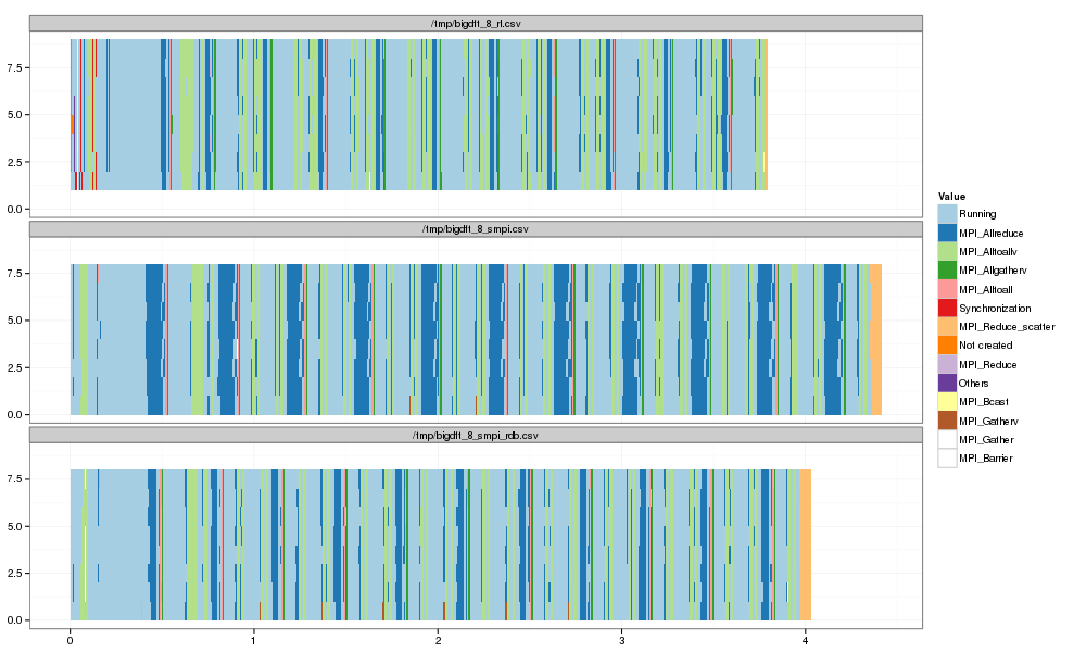
Fine. Now, let's make a Gantt Chart.
1 2 3 4 5 6 7 8 9 10 | |
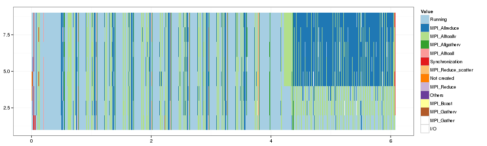
And voilà. Now, we have to compare it more finely with an SMPI trace…
First Comparison with SMPI
Let's try with one Augustin just sent me.
pj_dump $input | grep State | sed -e 's/PMPI/MPI/g' -e 's/rank-//' -e 's/computing/Running/' > $output
echo $output
/tmp/bigdft_8_smpi.csv
1 2 | |
  ResourceId    Start      End Duration       Value                 Origin
1          7 0.000000 0.000084 0.000084     Running /tmp/bigdft_8_smpi.csv
2          7 0.000084 0.000424 0.000340 MPI_Barrier /tmp/bigdft_8_smpi.csv
3          7 0.000424 0.000444 0.000020     Running /tmp/bigdft_8_smpi.csv
4          7 0.000444 0.000510 0.000066   MPI_Bcast /tmp/bigdft_8_smpi.csv
5          7 0.000510 0.000513 0.000003     Running /tmp/bigdft_8_smpi.csv
6          7 0.000513 0.000620 0.000107   MPI_Bcast /tmp/bigdft_8_smpi.csv
1 2 3 4 | |
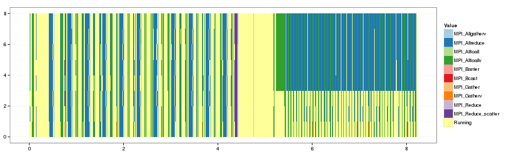
Let's plot them side by side
1 2 3 4 5 6 | |
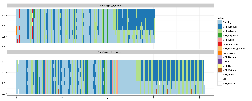
OK. That's a first step but obviously, our estimation of MPI_Allreduce
is quite pessimistic. It's likely to be explained by the fact that our
implementation of this collective in SMPI does not correspond at all to
the one of RL…
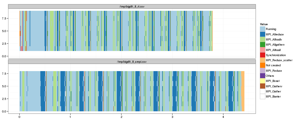
Mmmmh, let's limit to the first phase:
1 2 3 | |
And let's plot them side by side again
1 2 3 4 5 | |
Now, let's compare "state distributions".
1 2 3 4 5 6 7 8 | |
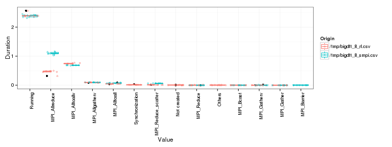
OK, so as expected the main difference lies in MPI_Allreduce. There is
also a small difference in MPI_Alltoallv and MPI_Reduce_scatter. The
other differences do not seem significant at this level of detail.
Using a "better" Allreduce implementation in SMPI
OK. Last attempt with a new trace that uses another implementation of
Allreduce.
/tmp/bigdft_8_smpi_rdb.csv
1 2 | |
Again, let's display them side by side:
1 2 3 4 5 6 | |
1 2 3 4 5 6 7 8 | |
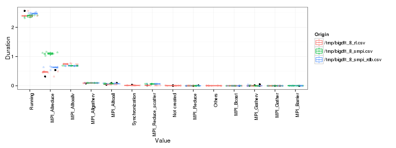
That's better. It's not perfect yet but it's improving and we may still not have the true algorithm…
Entered on [2013-04-03 mer. 11:36]